Introduction: This lab has been split into 2 major parts:

1. Analysis of simulated data
2. Experimental measurement of a thin turbid sample

Analysis of Simulated Data

A) How to use the GUI:

a) To launch the GUI interface used for this portion of the lab, locate the “IAD_simulated_data_GUI.m” in the “IAD lab” folder on the desktop. When Matlab opens, run this file from the editor window. The GUI should appear in a separate window.

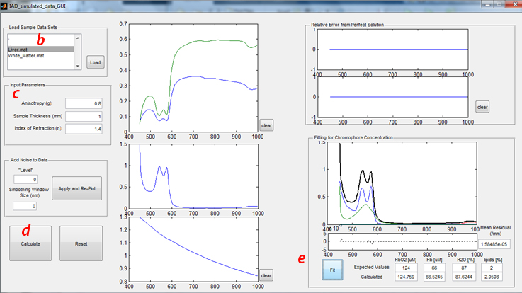
b) Load Sample Data Sets:

• Click “tissue types” in the upper left hand corner to select the desired tissue data (Liver.mat or White_Matter.mat). These two tissues were selected for this study, given their contrasting optical properties. Namely, liver tissue exhibits relatively high absorption and low scattering properties, whereas brain white matter is characterized by low absorption and high scattering.

1) Run through this sensitivity analysis procedure (including sections B and C) with both tissue types.

• Once the desired tissue is selected, Click the “load” button. The simulated Reflectance (Blue or Cyan) and Transmittance (Red or Magenta) spectra will appear in the figure immediately to the right of this panel.

c) Input Parameters

• In the panel below Load Sample Data Sets, the requisite sample input parameters are listed. For these exercises, all simulated data were generated with the following properties:

1) Sample thickness (physical thickness): 1mm

2) Index of refraction of the sample: 1.4

3) Scattering anisotropy (g): 0.8

d) Running the Inverse Adding-Doubling solver

• The “Calculate” button will submit the reflectance and transmittance spectra along with the input parameters into the IAD executable developed by Scott Prahl. Since this part of the lab uses simulated data, all the experimental considerations integrated in this executable have been disabled (which is not the case for the second part of this lab).
• This code will take a few seconds to run, but once completed:

1) The calculated absorption and reduced scattering coefficients will be plotted in the two figures below the Reflectance and Transmittance plot.

2) The error (% difference from ideal measurement as a function of wavelength) will be plotted in the top right figures. Using the correct input parameters will produce a 0% error, obviously.

e) Fitting Absorption Spectrum to determine Chromophore Concentration

• Clicking the “Fit” button in the lower right panel will perform a Linear Least-Squares operation, fitting the calculated absorption spectrum to the spectral response from oxy- (HbO2) and deoxy- (Hb), water (H2O), and Lipids. The expected values represent the concentrations of these 4 chromophores used to generated this simulated dataset.
• Even under idealized conditions such as these, the fits for these chromophores are not exact even though the model used here is an exact solution to the RTE. Can you speculate why?
• While the top figure in this panel shows the calculated absorption spectrum and the scaled basis spectra for the 4 chomophores as determined by the least-squares fit, the bottom figure shows the residual from this fit. The single value for the “Mean Residual” is the Sum of Residuals-Squared, divided by the number of data points in the spectrum.

f) Additional GUI features

• “Clear” buttons will clear the data from the adjacent figures
• “Reset” will clear all data loaded and plotted in the GUI
• “Add Noise” panel will be described later in “Effects of Measurement Noise” (section C)

B) Dependence (precision) of input parameters on the determination of Optical Properties and Chromophore concentration

1) Anisotropy: Tissue is typically described as having values of 0.7-0.99. It has also been documented that this value can slowly change as a function of wavelength over a large spectral range. However, when inverse solvers are used, a single invariant value for g is typically assumed and it is rarely measured directly from tissue.

• Change the value for Anisotropy in the Input Parameter panel to 0.7 and 0.9 and run the IAD solver at each value.
• How much error is accrued as a consequence of these erroneous values for g?
• How significantly does this alter the determination of chromophore concentrations? (keep the errors for each chromophore in mind going forward, as the determination of some chromophores concentrations may be more uncertain than others, and this may also be dependent on the composition of the tissue as well…)

2) Sample Thickness: From an experimental perspective there are a number of factors to consider in terms of what an "ideal sample thickness" would be (optical thickness (i.e., expected optical properties), balancing signal to noise in both Reflectance and Transmittance measurements, side light losses, etc., as well as your ability to precisely measure the sample thickness). These considerations matter even if you have the ability to prepare a tissue sample of a desired thickness.

• Change the sample thickness by +/- 10% and run IAD
• How are errors in sample thickness correlated with errors in the optical properties?
• How do these affect the chromophore concentrations?

3) Tissue Refractive Index: Like anisotropy, the refractive index of tissue is challenging to measurement determine. Moreover, it also varies gently with wavelength. Given the lack of experimental accessibility, this value is often assumed. In the context of IAD, it is useful to understand how this parameter can affect the calculation of optical properties and other downstream property determination, such as, chromophore concentrations.

• Change the index of refraction by +/- 10% and run IAD
• How are these changes in refractive index correlated with errors in the optical properties?
• How do these effect chromophore concentrations?

C) Effects of Measurement Noise (and post-processing methods to mitigate noise)

1) From the “Add Noise to Data” panel, you have the opportunity to alter the simulated reflectance and transmittance data in two ways:

• Add quasi- “signal-dependent” noise (mimicking typical measurement shot-noise). As we are starting with simulated calibrated data, the noise inserted here is arbitrary, but provides a sense for how raw measurement noise might propagate through the calibration process. To that end, the values used to “add noise” are somewhat arbitrary. For the purposes of this lab, use values of 5 and 10.
• Use a filtering method to smooth out the noise from the underlying signal. While there are a wide variety of filters that can be employed to signal process spectral measurements (all with their own strengths and weaknesses), a simple box-car filter is used in this lab. Here the “smoothing window size” represents the sliding spectral band used to average all data within that band in order to reduce the random noise in that window relative to the mean signal at each data point. Whereas a larger window would provide larger data sampling to minimize the variance from random noise, doing so would be at the expense of reducing the spectral resolution of the measurement.

2) Apply noise to the loaded data at levels of 5 and 10 and run the inverse solver. As noise is random, repeat this at least 3 times to better characterize the variance and consequences of this “level” of noise. Specifically, what becomes the variance in the chromophore concentration values?

3) At a noise level of 10, apply a smoothing window of 20 and 40nm (at least 3 times each)

• How do noise and smoothing affect the variance in the chromophore concentration values?
• Might these provide any apparent bias to the chromophore values? Is it tissue optical property specific?
• Can you think of any other way to improve this? (think in terms of smoothing, fitting, and/or chromophore reference spectra)

Experimental measurement of a thin turbid sample

There are two experimental setups provided to make measurements of thin turbid samples: a single sphere and a dual sphere configuration. The samples provided here are thin, tissue-simulating phantoms: silicone sheets embedded with titanium dioxide (as a scattering agent) and two sets of dyes (as the absorber). The computers attached to these systems have both the data acquisition code (LabView) and the data processing code (Matlab) specific to the components used in the respective setups. NOTE: these demo systems are NOT optimized for making robust IAD measurements, but rather are set up for instructional purposes.

A) About the samples

a) Thicknesses

•  These samples will vary slightly with spatial location. It is therefore important to select a specific sub region to measure with the integrating sphere and confirm that thickness with calipers and/or micrometers provided (the simulation portion of the lab will give some sense of errors due to misestimating thickness, but that does not reflect errors when the thickness varies between transmittance and reflectance measurements….)

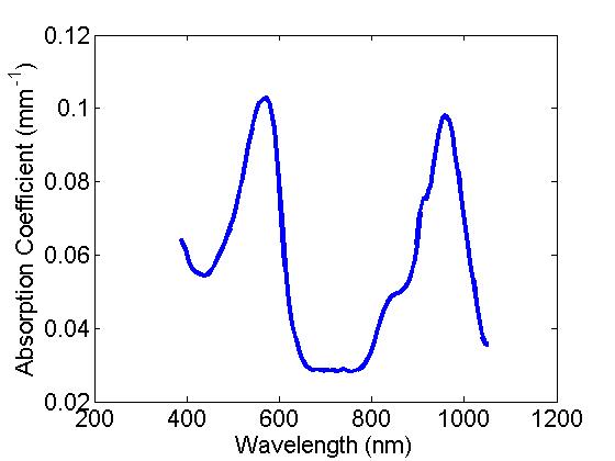
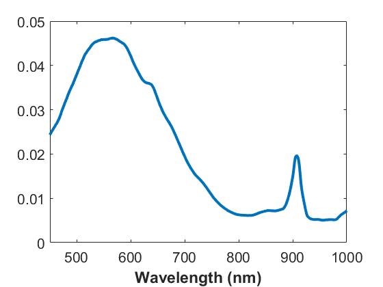
b) Optical Properties of these samples:

• Scattering: Titanium Oxide was used in both samples to provide tissue-like scattering properties. Commonly used in cosmetic products, this is an inert, fine white powder that contains a distribution of particle sizes that “looks like” scattering objects that typically scatter light in skin…
•  Absorption: Here a combination of two dyes provide a distinct spectral feature for the absorption of these samples with peaks at ~560 and ~970nm, or a single broad absorbing dye with a peak around 560 nm, basis spectra provided below:

B) Setup 1 (Single Sphere system)

a) Hardware description

• Light Source: 20W Quartz Tungsten Halogen lamp coupled via 100 micron optical fiber
• Beam collimation: 90 degree parabolic mirror collimates the light from the distal end of the fiber and an adjustable iris controls the spot size of the collimated beam (*NOTE-spot size has been set to 5mm and has been hard coded in the processing code, do not change the spot size for this exercise)
• Integrating sphere: 101.6mm diameter, with an entrance (transmission) port 19.05mm, an exit (reflectance) port 12.7mm, and detector port 6.35mm.
• Detection: from the detector port, a 400 micron fiber delivers the light to a BWTek spectrometer

b) Launching the Data acquisition GUI:

• In the “Lab E – IAD lab\Data Acquisition\” folder on the desktop, double click the IAD_acquire.vi to launch LabView.
• Make sure both light source and spectrometer are turned on
• Run the Labview GUI

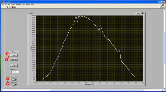
c) Data acquisition

• Spectral data acquisition procedure

1) With the system set up for any of the 3 measurements (calibration, transmittance, reflectance)

a. Click autoexpose button (this sets exposure time of the spectrometer to utilize the maximal available dynamic range of the detector without saturating *NOTE-this spectrometer is limited to go up to 65.5seconds)

b. Manually toggle the shutter to the closed position at the back of the lamp.

c. Click “Dark Noise” (this measures the background noise of the spectrometer and automatically subtracts this background from the subsequent measurement.

d. Open Shutter and click “Scan”. This will now acquire and plot the spectrum, dark noise corrected

e. Click “save data” to save the spectrum as a text file that will be submitted to the processing code.

• Note, you can generate a sub folder through this function to keep your files separate from other groups’ data
• There are 3 Types of measurements required to Process IAD data:

1) Sphere Calibration (essentially, this is the 100% transmittance reference measurement)

a. System Configuration

i. Entrance (transmittance) port open

ii. Exit (reflectance) port closed with white spectralon disk

2) Raw Sample Transmittance (detected integrated light that passes through the sample)

a. System Configuration

i. Sample placed flat against entrance (transmittance) port

ii. Exit (reflectance) port closed with white spectralon disk

3) Raw Sample Reflectance (detected integrated light that “diffusely reflects” from the sample)

a. System Configuration

i. Entrance (transmittance) port open

ii. Disk removed from Exit (reflectance) port; sample placed flat against exit port

C) Setup 2 (Dual Sphere system)

a) Hardware description

• Light Source: 20W Quartz Tungsten Halogen lamp coupled via 400 micron optical fiber
• Beam collimation: 90 degree parabolic mirror collimates the light from the distal end of the fiber and a second parabolic mirror brings it back to focus at the sample port of the fixed reflectance sphere.
• Integrating sphere: Two 76.2mm diameter spheres, with an entrance/sample ports 12.7mm and detector port 1 mm.
• Detection: from the detector ports, 400 micron fibers deliver the light to two Ocean Optics Flame spectrometers (Vis-NIR range)

b) Launching the Data acquisition GUI:

• Open folder called “Justin” on Desktop and click on DualSphereAcquisitionCode.vi to launch in labVIEW.
• Run the Labview GUI

c) Data Acquisition Procedure (3 parts - Acquire Data, Calibrate Transmittance, Calibrate Reflectance)

• Spectral data acquisition procedure

1) Place sample between reflectance and transmittance spheres, slide transmittance sphere toward reflectance sphere so that the sample is flush (and secure) between the two spheres’ ports

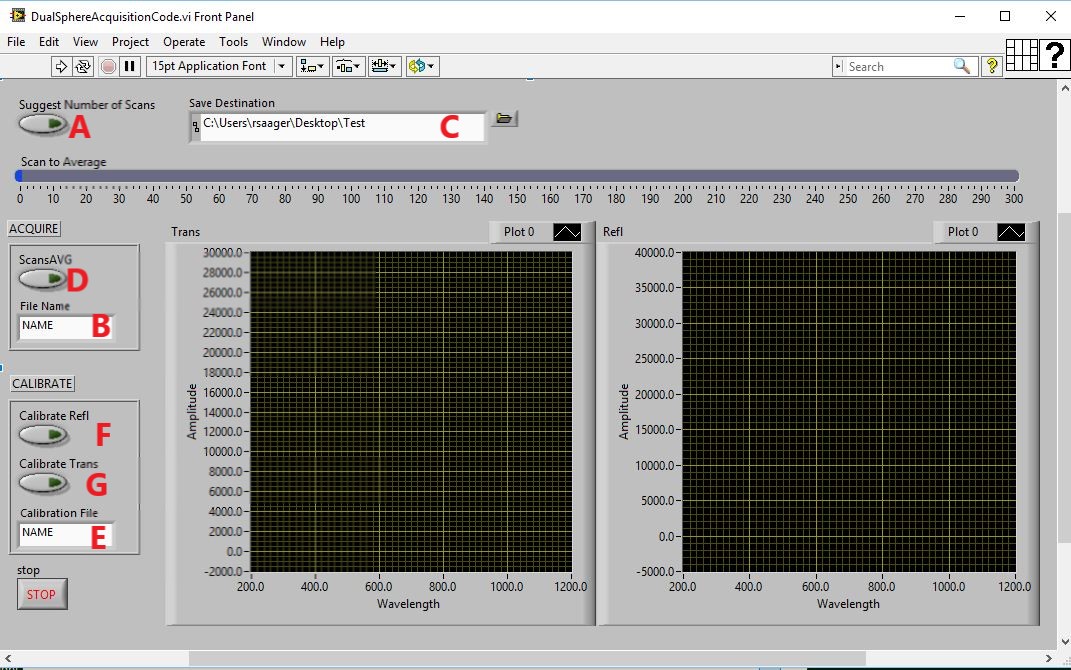
2) Click the Suggest Number of Scans button (A) after placing sample between spheres

3) Type descriptive file name for sample in the filename field (B) and ensure you have a save destination. (C)

• Click the ScansAVG button (D)

i. This will measure dark noise (closes shutter, waits, gets spectrum with set number of scans to average, and opens shutter)

ii. Acquires data subtracted by dark noise

iii. Auto saves with appended file names to differentiate reflectance from transmittance

• Calibration Sequence

All calibration data will be based on the filename used in field (E), but then appended to differentiate reflectance from transmittance

1) Reflectance (right sphere) uses calibration puck as sample

i. place between spheres and slide transmittance sphere to hold puck flat against the reflectance sphere port

ii. click Calibrate refl (F)

2) Transmittance (left sphere) uses the back of the sphere wall as a reference calibration

i. Slide transmittance sphere directly up against the reflectance sphere (no sample or calibration puck between the two spheres)

ii. Click Calibrate(G)

D) Data Processing

a) In the same folder double click the IAD_processing.m file (For system 1, use IAD_processingGTK.m, system 2: IADprocessing.m) to launch Matlab. In the editor window click run and the GUI should appear as a separate window.

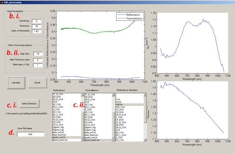
b) Input parameters

• Enter g (anisotropy), Thickness (in mm) and Index (n). For these silicone phantoms, g is assumed to be 0.9 and n is 1.43.

1. Other sphere parameters (sphere/port dimensions, beam diameter) have been hard coded in the data processing GUI.
2. Use calipers to measure the sample thickness and input it in the text box (units here are mm)

• Data processing step size: Prahl’s IAD code has extensively considered a wide variety of experimental non-idealities and means to identify and compensate for them. As a result, there is an additional layer of minimization (based on Monte Carlo) to ensure that the optical properties determined from IAD will also account for the physical realities of the measurement (e.g. light losses outside of the integrating sphere, etc). This can increase the processing time dramatically.

1. Setting the data processing step size reduces the number of spectral data points (running only every nth data point collected) to reduce the computational burden of the code. Recommend setting the step size to 10.

• Slide thickness, Slide Index: these parameters are used if you wish to calculate the optical properties of a sample contained in a cuvette (or sandwiched between glass slides)

1. As we are measuring bare silicone sheets, set the slide thickness to 0, and the slide index to 1 (matching air)

c) There are 3 list boxes, one for the raw reflectance, transmittance and sphere calibration measurements respectively.

• Clicking the Select directory button will let you choose the data folder that contains all your measurement data, clicking the highlighted text in one of the 3 list boxes will populate them with the filenames in this data directory
• Selected (by clicking) the appropriate measurement from the list for each measurement type

d) Enter a save file name at the left bottom and then Click the “Calculate” button and cross your fingers

• The above figure will plot the Calibrated Reflectance and Transmittance Spectra
• You can monitor the progress from the inverse solver in the command window of Matlab as it calculates the optical properties, wavelength by wavelength
• Up on completion, the figures to the right will plot the calculated optical properties (Absorption: Top, Scattering: Bottom)

e) Additional measurement parameters

• Beam diameter (defaulted in the processing code, so unless the iris is changed, it has been hard coded for 5mm)
• Sphere parameters: Sphere Size, Reflectivity, reflectance, transmittance and detector port sizes, etc have been determined in advance. (hard coded in the specific computers processing gui)

E) Discussion Questions

1 Do the resulting optical properties match your expectation for absorption and scattering?

• Does the absorption spectrum look like the provided spectra?
• Does scattering follow a monotonically (power-law like) decreasing trend?

2 From your sensitivity analysis in the simulated data section, can you infer where the most likely source of error may have come? (are these sample or instrumentation related?)

• and if so, what would you change to either verify and/or minimize this error?

3 Would you want to see an integrating sphere in your life …ever again?